This post will present a practitioner’s approach to analyzing asset allocation vs. manager selection effects on performance relative to the benchmark. The type of return attribution shown here is a geometric attribution. For a review of different types of attribution and the advantage of using geometric returns I’ll refer you to the CFA Institute’s literature review on Performance Attribution. One excerpt to highlight here is the history of the geometric approach: “Geometric models built on the idea of successive notional portfolios can be found in Holbrook (1977), Hymans and Mulligan (1980), and Allen (1991).
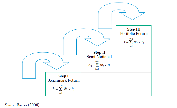
As shown in [the figure above], each successive portfolio represents an isolated decision in a top-down investment decision process. Step I represents the strategic, policy, or benchmark return. The difference between Step II and Step I represents the value added by active asset allocation, and the difference between Step III and Step II represents the value added by security selection. More steps can be introduced for more complex, multi-step investment decision processes.”
I refer to Step II, the Semi-Notional Portfolio, as an asset allocation portfolio. The weights equal the weights of the actual portfolio (Step III) but are implemented with benchmark indices instead of manager or security returns.
Example / Implementation
To illustrate let’s suppose we have a balanced portfolio with six actively managed mutual funds. We’ll set up initial weights to each fund at the beginning of 2023 and to illustrate asset allocation effects, we’ll rebalance to a more conservative portfolio in March 2023. To keep things simple the portfolio will consist of five asset groups: U.S. Large Cap, U.S. Small Cap, International Stocks, Emerging Market Stocks, and Core Bonds. Each manager gets a corresponding index: e.g., Fidelity Small Cap Discovery is mapped to the iShares Russell 2000 ETF and the Lord Abbett Core Plus is mapped to the iShares US Aggregate Bond ETF.
Finally to initiate the policy portfolio and analyze relative performance we’ll set up a 60 / 40 benchmark.
port <-data.frame(Manager =c('American Funds Washington Mutual Investors Fund','Fidelity Small Cap Discovery Fund','FMI International Fund','PIMCO RAE Emerging Markets Fund','Fidelity Total Bond Fund','Lord Abbett Core Plus'),Ticker =c('WSHFX', 'FSCRX', 'FMIJX', 'PEAFX', 'FTBFX', 'LAPLX'),Bench =c('IWB', 'IWM', 'EFA', 'EEM', 'AGG', 'AGG'),Weight =c(c(0.2, 0.2, 0.2, 0.05, 0.20, 0.15),c(0.15, 0.15, 0.15, 0.05, 0.30, 0.20)),Date =c(rep('2023-01-01', 6), rep('2023-03-15', 6)))port_bench <-data.frame(Ticker =c('IWB', 'IWM', 'EFA', 'EEM', 'AGG'),Weight =c(0.24, 0.06, 0.24, 0.06, 0.40),Date ='2023-01-01')port
                                           Manager Ticker Bench Weight
1  American Funds Washington Mutual Investors Fund  WSHFX   IWB   0.20
2                Fidelity Small Cap Discovery Fund  FSCRX   IWM   0.20
3                           FMI International Fund  FMIJX   EFA   0.20
4                  PIMCO RAE Emerging Markets Fund  PEAFX   EEM   0.05
5                         Fidelity Total Bond Fund  FTBFX   AGG   0.20
6                            Lord Abbett Core Plus  LAPLX   AGG   0.15
7  American Funds Washington Mutual Investors Fund  WSHFX   IWB   0.15
8                Fidelity Small Cap Discovery Fund  FSCRX   IWM   0.15
9                           FMI International Fund  FMIJX   EFA   0.15
10                 PIMCO RAE Emerging Markets Fund  PEAFX   EEM   0.05
11                        Fidelity Total Bond Fund  FTBFX   AGG   0.30
12                           Lord Abbett Core Plus  LAPLX   AGG   0.20
         Date
1  2023-01-01
2  2023-01-01
3  2023-01-01
4  2023-01-01
5  2023-01-01
6  2023-01-01
7  2023-03-15
8  2023-03-15
9  2023-03-15
10 2023-03-15
11 2023-03-15
12 2023-03-15
The code snippet below downloads the returns from tiingo. If you want to follow along / reproduce this example you can follow the link to register for a free api key. I’ve hidden mine, so you will need to set the variable t_api below to your api key. The ending result ret is the time-series of returns for all the benchmarks and active managers needed to create the portfolios.
A quick note on data structures before describing the rebalance / contribution to return algorithm: I will use the term matrix below to describe many of the data such as the return matrix, the asset weight matrix, the asset wealth matrix, etc. However, the technical R implementation I use is an xts or extensible time-series. The xts is essentially a matrix and allows us to mathematically operate on the data like a matrix while keeping the meta-data of each row representing a date or time.
Rebalance Portfolios
This is the key section for implementing. We need a rebalance function to calculate the portfolio’s return and the geometric contribution to return for each asset. The function will take two inputs:
ret is the matrix of returns, for the our example the returns are
Both ret and wgt have the same number of columns that correspond to each asset. ret will have a row for every day there are returns, while wgt will not necessarily have a rebalance each day, in our example there are only two rebalances and 1,945 days of returns.
To keep track of the geometric returns we’ll set up an asset_wealth matrix with corresponding columns to ret and wgt and one extra row to account for the initial wealth value. We also need the matrix of asset weights, asset_wgt, with the same corresponding columns and rows to ret.
asset_wgt represents the beginning of the day’s asset weights while asset_wealth represents the end of the day’s wealth. The ret is the day’s return that grows (or decreases) the asset_wealth. Note that since the asset_wealth is lagged, at day i, the asset_wealth[i, ] is the previous day’s ending value and corresponds to the same day as asset_wgt[i-1, ].
The rebalance algorithm is as follows:
Loop through each day, i, in the return matrix
If we need to rebalance based on the rebalance weights, wgt, then:
Set the asset weight matrix, asset_wgt[i, ] at the rebalance day i to the rebalance weights at day i.
Else, we don’t need to rebalance.
Set the asset_wgt[i, ] to the percent of each asset’s wealth relative to the total portfolio wealth of the previous day: asset_wealth[i, ] / sum(asset_wealth[i, ]).
Grow the asset wealth at the end of day i by compounding the return of at day i multiplied by the asset weight at the beginning of day i: asset_wealth[i + 1, ] <- sum(asset_wealth[i, ]) * asset_wgt[i, ] * (1 + ret[i, ]).
This completes the rebalance. The row sums of the asset_wealth matrix will give us the portfolio wealth time-series, which easily be converted to returns by taking the % day over day change. To calculate the contribution to return by asset we’ll set up a contribution to return matrix, ctr_mat with corresponding columns and rows to ret. For each day i the contribution to return at day i is portfolio wealth at the end of the previous day * the return of day i * the beginning weight of day i: ctr_mat[i, ] <- sum(asset_wealth[i, ]) * asset_wgt[i, ] * r[i, ]. The column sums of the ctr_mat / the initial portfolio wealth of 100 will equal the return contributions for each asset. The contributions will sum to the total portfolio geometric return for the corresponding period.
library(lubridate)library(tidyr)rebal <-function(ret, wgt) {# subset ret xts to the desired tickers in our portfolio r <- ret[, match(colnames(wgt), colnames(ret))]# start returns at first rebalance date r <- r[paste0(zoo::index(wgt)[1], '/')]# asset wealth matrix to track $ value of each asset# at the end of each day asset_wealth <-matrix(nrow =nrow(r) +1, ncol =ncol(r))# start with $100 before first return at time 0 asset_wealth[1, ] <-as.numeric(wgt[1, ]) *100# asset wgt matrix tracks weight of # the assets at the beginning of each day asset_wgt <-matrix(nrow =nrow(r), ncol =ncol(r)) asset_wgt[1, ] <-as.numeric(wgt[1, ]) dt_vec <- zoo::index(r) reb_counter <-2# loop through each day ifor (i in1:nrow(r)) {# check if we are at or just missed a rebalance dateif (reb_counter <=nrow(wgt) & dt_vec[i] >= zoo::index(wgt)[reb_counter]) {# rebalance portfolio by setting beginning period weight# to our rebalane weight asset_wgt[i, ] <-as.numeric(wgt[reb_counter, ]) reb_counter <- reb_counter +1 } else {# if not on rebalance period the beginning weight# is the previous day's ending value / the total asset_wgt[i, ] <- asset_wealth[i, ] /sum(asset_wealth[i, ]) }# grow the wealth by the beginning period weights and# the day's return asset_wealth[i +1, ] <-sum(asset_wealth[i, ]) * asset_wgt[i, ] * (1+ r[i, ]) }# set up contribution to return matrix ctr_mat <-matrix(nrow =nrow(r), ncol =ncol(r))# for each period contribution to return is # port wealth at beginning * asset weight at beginning *# forward asset return for the periodfor (i in1:nrow(r)) { ctr_mat[i, ] <-sum(asset_wealth[i, ]) * asset_wgt[i, ] * r[i, ] } ctr_df <-data.frame(Asset =colnames(r), Contr.to.Return =colSums(ctr_mat) /100)# load our data into a list and return the results res <-list() res$ctr_df <- ctr_df res$port_wealth <-xts(rowSums(asset_wealth), c(dt_vec[1] -1, dt_vec)) res$port_ret <- res$port_wealth /lag.xts(res$port_wealth, 1)[-1, ] -1return(res)}
The weights need to be restructured from the data.frames to a xts matrix and then we can run the rebal function. The mgr_wgt represents the actual portfolio (Step III) and the asset_wgt represents the asset allocation or semi-notional portfolio (Step II). The bench_wgt is the benchmark or policy portfolio (Step I).
Let’s check the results of the portfolio to see if the sum of the return contribution equals the total portfolio return. We can also plot the portfolio’s wealth value or cumulative geometric return over time to see if it looks reasonable.
The benchmark return was 4.29%, during this time-period nearly all the returns came from stocks, and U.S. stocks drove more return than their International counterparts.
The first attribution to determine the asset allocation effects is calculated by the asset allocation portfolio’s return contribution less the benchmark’s return contribution. The subtraction is element by element for corresponding asset classes. In the case of two bond managers having the same AGG index we can combine the two AGG indices in the asset allocation portfolio to correspond to the one AGG index in the benchmark.
The portfolio sold out of stocks and into bonds before a period of positive stock performance and negative bond performance: we expect the asset allocation decisions to be negative.
The asset allocation portfolio returned 2.75% which detracted 1.54% relative to the benchmark. The Asset.Perf column shows the returns of each asset after the portfolio rebalance from stocks to bonds. Bonds had a negative return so it makes sense their attribution is negative. The Small Cap attribution is positive. This may seem counterintiutive, although the post rebalance returns were negative, Small Caps had a slightly positive performance for the total time-period and a larger weight than the benchmark. However, most allocators would consider the decision to weight Small Caps in concert with their Large Cap counterparts, which outperformed during this period. The attribution is additive so when you combine the Small Cap and Large Cap into one tactical component, this Small / Large Cap “trade” or “leg” detracted 0.83% from the benchmark.
The manager performance added 1.47% of performance. Since the 3/15 rebalance all of the managers except for Large Cap outperformed their benchmarks which matches the direction of the attribution. The totals square: the benchmark return of 4.29% minus 1.54% of asset allocation effect plus 1.47% of manager selection equals the portfolio return of 4.22%. In hindsight we knew the allocation decision of selling Stocks and buying Bonds in March hurt as well as being overweight Small Cap. But if we just looked at the performance of the portfolio relative to the benchmark we would only see a 7 bps difference. Obviously a significant portion of the underperformance was offset by manager selection and we might have an intuition that this happened but it’s important to be able to quantify to what extent so we can properly judge both parts of the investment process.
Astute readers will point out there’s an interaction effect that is getting “swept” up in the selection effect when we subtract the asset allocation portfolio from the actual portfolio. While there are algorithms to break it out, I prefer to keep things simple and have portfolios that tie to an economic hypothetical. The three step approach allows you to ask what if we didn’t make asset allocation decisions and just tried to win on manager outperformance or vice versa.
Lastly I’ll expand on the flexibility of this framework highlighted in the introduction. For example, maybe your investment process makes equity allocation decisions at the total U.S. vs. ex-U.S. level and then within U.S. there are managers with various Growth, Value, Large Cap, Small Cap, etc, mandates that aren’t explicitly part of the asset allocation decision. You could create a high level asset allocation portfolio with all the U.S. managers under the Russell 3000 and then another semi-notional portfolio with all the sub-asset class benchmarks for the underlying managers to judge if there is a significant benchmark mismatch effect within U.S. equities (and the other broader asset classes as well). This approach could nicely complement a tracking error risk budget to see where risk was being taken and how it paid off.